Human Thymus Multimodal Deconvolution
This tutorial demonstrates multimodal deconvolution on simulated human thymus spatial data derived from a single-cell multiomic (CITE-seq) dataset with paired RNA and protein (ADT) measurements.
The single-cell multiomic dataset contains 11 batches, which are paired to form 11 batch-pair datasets. Within each pair, one batch is used as the reference and the other is used to simulate spatial data. The simulation scheme follows the idea described in Spatial transcriptomics deconvolution methods generalize well to spatial chromatin accessibility data.
Datasets are available on Zenodo.
[ ]:
import muon as mu
import os
from os.path import join
import scanpy as sc
import pandas as pd
import numpy as np
import matplotlib.pyplot as plt
import glob

import sparank
from sparank.config import ExpConfig, ModalityConfig, SimulationConfig
from sparank.framework import SpaRank
[2]:
data_dir = '../data/human_thymus/simulated'
batch_pairs  = pd.read_csv(f'{data_dir}/batch_pairs.csv')
Training
The cell below shows the training configuration used in our experiments. It is commented out by default, so you only need to run it if you want to reproduce the models from scratch.
A few settings are worth noting:
modalities=[ModalityConfig(name="rna", ...), ModalityConfig(name="adt", ...)]: specific configurations for RNA and protein modalities.context_key=None: no context conditioning is used.
[3]:
# for (spot_batch, cell_batch) in zip(batch_pairs.spot, batch_pairs.cell):
#     pair_id = f'{spot_batch}-{cell_batch}'

#     mdata_ref = mu.read_h5mu(
#         glob.glob(join(data_dir, f'{cell_batch}-*', "ref_data.h5mu"))[0]
#     )
#     adx_sc_rna = mdata_ref.mod['rna']
#     adx_sc_adt = mdata_ref.mod['adt']

#     adx_sc_rna.var_names_make_unique()
#     adx_sc_adt.var_names_make_unique()

#     cfg = ExpConfig(
#         modalities=[
#             ModalityConfig(name="rna", top_k=500, cl_dropout_rate=0.3, mrp_mask_rate=0.3),
#             ModalityConfig(name="adt", top_k=500, cl_dropout_rate=0.3, mrp_mask_rate=0.3)  # top_k will subset to the actual protein panel
#         ],
#         simulation=SimulationConfig(
#             total_samples=500_000,
#             batch_request_size=100_000,
#             batch_key='sample',
#         ),
#         celltype_key='annotation',
#         batch_key='sample',
#         context_key=None,
#         dim=128,
#         depth=2,
#         heads=4,
#         cl_weight=0.5,
#         cl_temperature=0.1,
#         mrp_weight=0.5,
#         cls_weight=1.0,
#         epochs=20,
#         num_workers=0
#     )

#     model = SpaRank(cfg=cfg, save_dir=f'../outputs/human_thymus/{pair_id}')
#     model.register_modality("rna", adx_sc_rna)
#     model.register_modality("adt", adx_sc_adt)
#     model.prepare()    # use sp gene panel as a prior
#     model.fit()              # train
#     model.save()

#     break
Evaluation
After training, we load the checkpoint and apply it to the corresponding simulated spatial sections. The predicted cell-type proportions are then compared against the ground truth from simulation.
We report Jensen–Shannon divergence and Pearson correlation scores to assess deconvolution performance. We also track modality gate scores to examine how the model balances RNA and ADT signals.
[4]:
from typing import Union

import numpy as np
import pandas as pd
from scipy.spatial.distance import jensenshannon
from scipy.stats import pearsonr

def _to_array(x):
    return x.values if isinstance(x, pd.DataFrame) else np.asarray(x)

def jsd(true: Union[pd.DataFrame, np.ndarray], predicted: Union[pd.DataFrame, np.ndarray]) -> float:
    jsd_vals = jsd_per_col(true, predicted)
    return np.nanmean(jsd_vals)

def jsd_per_col(true: Union[pd.DataFrame, np.ndarray], predicted: Union[pd.DataFrame, np.ndarray]) -> np.ndarray:
    t = _to_array(true)
    p = _to_array(predicted)

    n_cols = t.shape[1]
    vals = np.full(n_cols, np.nan, dtype=float)
    for i in range(n_cols):
        a = t[:, i].astype(float)
        b = p[:, i].astype(float)
        sa = a.sum()
        sb = b.sum()
        if sa == 0 or sb == 0:
            vals[i] = np.nan
            continue
        pa = a / sa
        pb = b / sb
        vals[i] = float(jensenshannon(pa, pb, axis=0, base=2))
    return vals


def pcc(true: Union[pd.DataFrame, np.ndarray], predicted: Union[pd.DataFrame, np.ndarray]) -> float:
    r_vals = pcc_per_col(true, predicted)
    return float(np.nanmean(r_vals))


def pcc_per_col(true: Union[pd.DataFrame, np.ndarray], predicted: Union[pd.DataFrame, np.ndarray]) -> np.ndarray:
    t = _to_array(true)
    p = _to_array(predicted)

    n_cols = t.shape[1]
    vals = np.full(n_cols, np.nan, dtype=float)
    for i in range(n_cols):
        x = t[:, i]
        y = p[:, i]
        if np.std(x) == 0 or np.std(y) == 0:
            vals[i] = np.nan
            continue
        vals[i], _ = pearsonr(x, y)
    return vals


def eval_pred(targets, pred):

    jsd_mean_row = jsd(targets.T, pred.T)  # by row
    pcc_mean_row = pcc(targets.T, pred.T)
    jsd_mean_col = jsd(targets, pred)  # by row
    pcc_mean_col = pcc(targets, pred)

    d = {
        'jsd-mean-row': jsd_mean_row,
        'pcc-mean-row': pcc_mean_row,
        'jsd-mean-col': jsd_mean_col,
        'pcc-mean-col': pcc_mean_col,
    }
    return d
Metrics
[5]:
import torch

rs = []
gate_scores = {}
for (spot_batch, cell_batch) in zip(batch_pairs.spot, batch_pairs.cell):
    pair_id = f'{spot_batch}-{cell_batch}'

    model = SpaRank.load(f'../outputs/human_thymus/{pair_id}', device="cuda:0")
    mdata_sp = mu.read_h5mu(
        glob.glob(join(data_dir, f'{spot_batch}-*', "sp_data.h5mu"))[0]
    )

    adx_sp_rna = mdata_sp.mod['rna']
    adx_sp_adt = mdata_sp.mod['adt']

    adx_sp_rna.var_names_make_unique()
    adx_sp_adt.var_names_make_unique()

    gate_scores[pair_id] = []
    for ep in np.arange(model.cfg.epochs):
        ckpt = join(model.save_dir, f"model_epoch{ep+1}.pth")
        model.model.load_state_dict(torch.load(ckpt, map_location=model.device))

        preds, gates = model.predict(mod_adatas={'rna':adx_sp_rna, 'adt':adx_sp_adt}, return_gate_scores=True)
        df_true = pd.DataFrame(adx_sp_rna.obsm['proportions'],
                           columns=adx_sp_rna.uns['proportion_names']).copy()
        df_pred = preds.reindex(columns=df_true.columns, fill_value=0)

        df_true = df_true.div(df_true.sum(axis=1), axis=0)
        df_pred = df_pred.div(df_pred.sum(axis=1), axis=0)
        rna_r = eval_pred(df_true, df_pred)
        rna_r['dataset'] = pair_id
        rna_r['ep'] = ep + 1

        # print(ep, rna_r)
        rs.append(rna_r)
        gate_scores[pair_id].append(gates.mean(axis=0)[0])

    break
[6]:
df_res = pd.DataFrame(rs)
df_res
[6]:
| jsd-mean-row | pcc-mean-row | jsd-mean-col | pcc-mean-col | dataset | ep | |
|---|---|---|---|---|---|---|
| 0 | 0.620966 | 0.422434 | 0.547996 | 0.498087 | TT-CITE-1-TT-CITE-5 | 1 |
| 1 | 0.585704 | 0.506616 | 0.538801 | 0.522315 | TT-CITE-1-TT-CITE-5 | 2 |
| 2 | 0.542583 | 0.595207 | 0.524391 | 0.572617 | TT-CITE-1-TT-CITE-5 | 3 |
| 3 | 0.530953 | 0.616906 | 0.513516 | 0.593068 | TT-CITE-1-TT-CITE-5 | 4 |
| 4 | 0.521424 | 0.630698 | 0.506310 | 0.619039 | TT-CITE-1-TT-CITE-5 | 5 |
| 5 | 0.508718 | 0.642302 | 0.501077 | 0.636270 | TT-CITE-1-TT-CITE-5 | 6 |
| 6 | 0.507621 | 0.642506 | 0.494738 | 0.651287 | TT-CITE-1-TT-CITE-5 | 7 |
| 7 | 0.521434 | 0.614370 | 0.496680 | 0.651511 | TT-CITE-1-TT-CITE-5 | 8 |
| 8 | 0.511970 | 0.618444 | 0.488771 | 0.661643 | TT-CITE-1-TT-CITE-5 | 9 |
| 9 | 0.495957 | 0.649375 | 0.484811 | 0.663655 | TT-CITE-1-TT-CITE-5 | 10 |
| 10 | 0.505268 | 0.631040 | 0.484866 | 0.667103 | TT-CITE-1-TT-CITE-5 | 11 |
| 11 | 0.497875 | 0.639952 | 0.484147 | 0.666498 | TT-CITE-1-TT-CITE-5 | 12 |
| 12 | 0.515348 | 0.606359 | 0.494060 | 0.645583 | TT-CITE-1-TT-CITE-5 | 13 |
| 13 | 0.507942 | 0.630888 | 0.487754 | 0.666721 | TT-CITE-1-TT-CITE-5 | 14 |
| 14 | 0.499108 | 0.633821 | 0.484229 | 0.662645 | TT-CITE-1-TT-CITE-5 | 15 |
| 15 | 0.504156 | 0.623252 | 0.484261 | 0.663488 | TT-CITE-1-TT-CITE-5 | 16 |
| 16 | 0.498450 | 0.632995 | 0.485791 | 0.663203 | TT-CITE-1-TT-CITE-5 | 17 |
| 17 | 0.497066 | 0.632111 | 0.484906 | 0.657270 | TT-CITE-1-TT-CITE-5 | 18 |
| 18 | 0.509916 | 0.616092 | 0.486829 | 0.661512 | TT-CITE-1-TT-CITE-5 | 19 |
| 19 | 0.497279 | 0.638984 | 0.485762 | 0.666644 | TT-CITE-1-TT-CITE-5 | 20 |
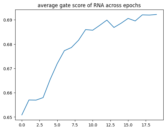
Modality ate score
The plot below shows the average RNA gate score across training epochs for one dataset, illustrating how the model weights the RNA modality during optimization.
[7]:
# pair_id = 'TT-CITE-1-TT-CITE-5'

plt.plot(gate_scores[pair_id])
plt.title('average gate score of RNA across epochs')
[7]:
Text(0.5, 1.0, 'average gate score of RNA across epochs')
[ ]: